
Hello Potato World
[포테이토 스터디] Pixel Attribution (Saliency Maps) 본문
⋆ 。 ˚ ☁︎ ˚ 。 ⋆ 。 ˚ ☽ ˚ 。 ⋆
[XAI study_ Interpretable Machine Learning]
7.2 Pixel Attribution (Saliency Maps)
(비슷한 의미로 불리는 용어들)
Pixel attribution = Sensitivity map = Saliency map = Pixel attribution map = Gradient-based attribution method = Feature relevance = Feature attribution = Feature contribution
- 두 가지의 다른 방식의 Attribution
1. Feature attribution Methods
prediction이 얼마나 변화했는지에(Negatively/Positively) 따라 각 input feature를 평가
Feature는 pixel, tabular, word data가 input이 될 수 있음
SHAP, Shapley Vales, LIME 이 대표적인 예시
2. Pixel Attribution Methods
이미지 데이터를 위한 Feature attribution의 special case
Neural network에 의한 이미지 classification에 연관된 픽셀들을 강조하는 method
- 2 different types of Pixel attribution methods
(매우 많은 methods중 두개만 소개)
1. Occlusion- or perturbation-based method
SHAP나 Lime처럼 이미지의 일부를 조작하여 explanation을 만드는 방식 (model-agnostic)
2. Gradient-based method
input feature에 대한 prediction의 Gradient를 계산하여 explanation을 만드는 방식
=> 두 방식의 공통점
- explanation이 input image와 동일한 크기를 가짐
- 각 픽셀마다 prediction과의 연관성을 해석해서 값을 지정할 수 있음
(그 이외의 다양한 method들을 구분하는 기준들)
3-(1) Gradient-only methods
한 픽셀에서의 변화가 prediction을 바꾸는지를 분석
- (ex) Vanilla Gradient, Grad-CAM
3-(2) Path-attribution methods
Current Image(실제 예측)와 Reference Image(기준 예측)의 차이를 구해서 픽셀 단위로 나누는 것
Baseline Image(=Reference Image) : 한장의 이미지 또는 여러장(이미지 분포)이 될 수 있음
- (Model-specific example) Deep Taylor, Integrated Gradients
- (Model-agnostic example) LIME, SHAP
7.2.1 Vanilla Gradient (Saliency Maps)
- pixel attribution approaches
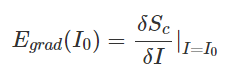
각 input 픽셀에 대해서 구하고자 하는 class의 Loss function의 Gradient를 계산
Output은 negative/positive 값들도 채워진 input feature과 동일한 크기의 map
- Approach :
1. 이미지에 대해 forward pass를 수행
2. input pixel에 대해 구하고자 하는 class score의 Gradient를 계산
3. 계산된 Gradient 시각화
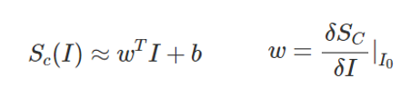
비선형적 function이 포함된 계산을 바로 할 수 없기 때문에 First-order Taylor expansion을 적용하여 score를 근사화하려는 아이디어
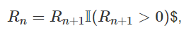
ReLU와 같은 비선형적인 unit이 sign을 제거해서, Backpass를 수행할 때 분석이 어려울 수 있음
element-wise indicator function I를 사용
- I : 이전 layer의 activation값이 음수면 0, zero나 양수면 1
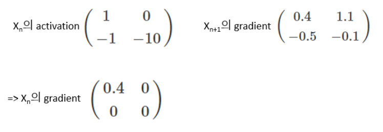
- 이전 layer의 활성화값이 음수면 gradient를 0으로 설정
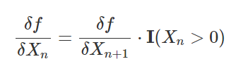
- Backpass example (n->n-1)
7.2.2 DeconvNet
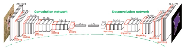
Neural Network를 거꾸로 뒤집는 방법
논문에서 filtering, pooling, activation layer를 뒤집는 공식을 제안
나머지 부분은 Vanilla Gradient와 동일하고, ReLU로 전달되는 gradient를 선택하는 방식만 다름
layer n의 activation중에서 forward pass시에 0이였던 것을 기억해서 layer n-1에서도 0으로 설정
layer n에서 음수값을 가지는 activation도 layer n-1에서 0으로 설정
- Backpass example (n->n-1)

7.2.3 Grad-CAM (Gradient-weighted Class Activation Map)
CNN prediction에 대한 시각적인 설명을 제공
다른 방법들처럼 모든 layer에 대해 backpropagated하는게 아니라, 마지막 convolutional layer에만 수행해서 이미지의 중요한 영역만 강조하는 map을 생성
- Grad-CAM의 Goal : Convolutional layer가 이미지를 분류하기 위해 해당 이미지의 어떤 부분을 보는지 이해하는 것
(보통 CNN의 과정)첫 번째 Convolutional layer는 input이미지를 받아서 학습한 특징들을 output feature maps으로 encoding하고, 다음 layer들은 이전 layer의 feature map을 받아서 동일한 작업 수행
여기서 Grad-CAM은 마지막 Convolution layer의 feature map의 어떤 부분이 활성화되는지 분석
- 마지막 Convolutional layer가 $𝐴_1,𝐴_2,...,𝐴_𝑘$ 총 k개의 feature map을 가지고 있을 때 (두 가지 방법)
1. feature map 그대로를 시각화해서 평균화하고, input image에 겹치는 방법
feature map 전체를 사용하면 모든 class에 대한 정보를 가지고 있기 때문에 적합하지 않을 수 있음
2. 평균화하기 전에, feature map의 pixel마다 각각의 gradient만큼의(class c에 대한) 가중치를 부여하는 방법
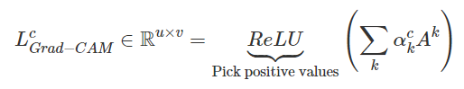
class c에 대해 positively or negatively 영향을 주는 영역을 강조하는 heatmap 생성
이 heatmap이 ReLU function을 통과해서, 모든 음수가 0으로 설정됨
(음수값을 제거하고 class c의 예측에 기여하는 영역들만 남음)
이 Grad-CAM map을 [0,1]범위로 조정한 후에 input image에 겹침
- Approach:
아래와 같이 정의된 localization map
1.input image에 대해 Convolutional Neural Network에서 forward propagate 수행
2. Softmax layer를 통과하기 전 Neuron의 activation(class c에 대한 raw score)을 얻음
3. 모든 class activation을 0으로 설정
4. fully connected layer 이전의 마지막 convolutional layer에서 class c에 대한 gradient를 backpropagate함
5. feature map의 각각의 pixel에 class에 대한 gradient값으로 가중치를 부여한다.
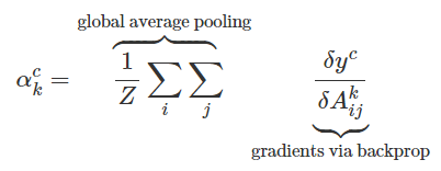
6. 부여된 가중치를 사용하여 Feature map들의 평균을 계산한다.
7. 평균화된 Feature map에 대해 ReLU함수를 적용한다.
8. 시각화를 하기 위해: 모든 값을 0-1사이로 scaling하고, 원본 이미지에 겹친다.
7.2.4 Guided Grad-CAM
Grad-CAM은 마지막 Convolutional layer만 사용하는데, 여기서의 Feature map은 원본 이미지보다 훨씬 coarse하기 때문에 localization도 디테일하지 못할 수 있다.
- Approach :
1. Grad-CAM explanation 계산
2. 각 pixel에 대해 모든 계층을 Backpropagation하는 방법을 사용하여 explanation 계산(ex. Vanilla Gradient)
3. 개별적으로 계산된 두 map을 곱함
Grad-CAM이 특정 class, pixel의 특정 부분에 초점을 맞추는 렌즈의 역할을 할 수 있음
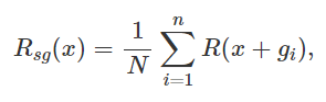
7.2.5 SmoothGrad
Noise를 인공적으로 추가하고 평균화하는 방식으로, noise를 줄이는 explanation
- Approach :
1. 이미지에 noise를 추가해서 여러 장의 input image를 생성
2. 모든 이미지에 대해 pixel attribution map을 생성
3. 모든 pixel attribution map을 평균화
gradient에 조금만 변동이 생겨도 결과가 크게 흔들리기 때문에, 여러 이미지를 통해 Gradient를 smoothing하는 효과를 내기 위함
7.2.6 Example
Examination for VGG-16, trained on ImageNet (highest classification score)
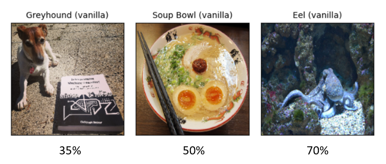
classification에 대한 explanation을 위해 생성한 pixel attributions:
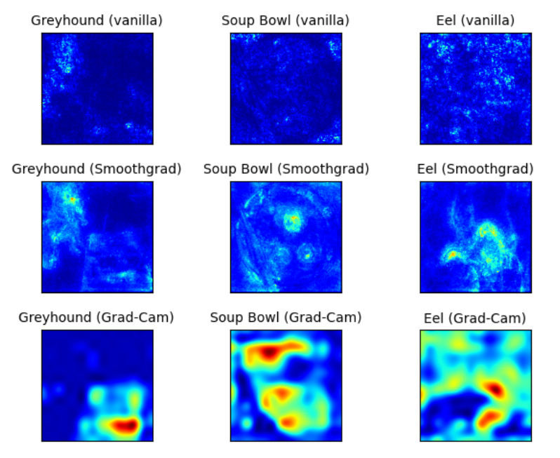
- 첫번째 이미지
Vanilla와 Smoothgrad는 강아지를 올바르게 highlight하기 했지만, 책도 일부 highlight됨
Grad-Cam은 거의 책만 highlight됨
- Vanilla Gradient는 Soup bowl과 Octopus 둘 다 highlight 실패
SmmothGrad는 최소한 영역(위치)을 알아보는 데라도 성공
Grad-CAM은 Soup Bowl은 어느정도 재료들 위치를 highlight했지만, Octopus는 엉망
7.2.7 Advantages
- explanation이 visual해서 이미지를 빠르게 인식할 수 있다.
method가 중요한 영역만 잘 highlight했을 경우, 중요한 영역을 빨리 알아채기 쉽다. - Gradient기반의 method들은 model-agnostic method들보다 계산 속도가 빠르다.
ex) SHAP와 LIME을 이미지 분류를 설명하기 위해 사용하면 계산량이 매우 클 것이다. - 선택할 수 있는 Method종류가 많다
7.2.8 Disadvantages
- 다른 해석방법들처럼 explanation이 정확한지 알 수 없다.
- Pixel attribution methods는 아직 매우 약해서 다른 픽셀들이 highlight되는 경우가 많다
- explanation의 신뢰도가 매우 떨어진다는 실험 결과가 있음
이미지의 모든 픽셀에 같은 변환을 주고 실험해본 결과, 단순 constant shift로 prediction은 바뀌지 않았지만 explanation이 변한 걸 볼 수 있었다. - 전반적으로 이 방법이 매우 불안정하고 부정확하기 때문에 이 방법들을 평가하는 연구들을 더 기다려야 한다...
References
[1] Interpretable Machine Learning, Christoph Molnar
'Study > XAI' 카테고리의 다른 글
| [포테이토 스터디] LRP: Layer-wise Relevance Propagation (0) | 2021.08.02 |
|---|---|
| [포테이토 스터디] Detecting Concepts (0) | 2021.06.28 |
| [포테이토 스터디] Influential Instances (0) | 2021.06.22 |
| [포테이토 스터디] Prototypes and Criticisms (0) | 2021.06.22 |
| [포테이토 스터디] Local Surrogate(LIME) (0) | 2021.05.24 |


